【備忘録】PsychoPy + アイトラッカー(例:Tobii)で眼球運動計測
本記事について
タイトルのとおり,PsychoPy + アイトラッカー(例:Tobii)で眼球運動計測する際の手順を自分のためにメモしたもの.もし誤りや,より良い方法があれば,ご教示ください.
なお現在のところ,PsychoPy Builderで実験を作ることを仮定しています.2026/7/3時点の最新バージョンである,バージョン2026.1.3を使用しています.
実験の作成
まず次の公式ページのとおり,PsychoPy内で使用予定のアイトラッカーのプラグインをインストールしてください.
次にこの動画のとおり,Builderで実験を作ります.
- Calibrationコンポーネント
- Validationコンポーネント
- Recordingコンポーネント
の順に,それぞれをルーティンとして配置します.
なおTobiiを使用する際は,プロパティ(歯車アイコン)でTobii Technology (iohub)を選びます.以下の動画では7:11~のメニュー.
特に重要なのは,眼球運動計測が行われるルーティンの開始・終了時点で,フラグを立てることです.以下の動画の,3:20~のとおり,codeコンポーネントで,
Begin RoutineioServer.sendMessageEvent(text = 'trial_start', category = 'custom_marker')
End RoutineioServer.sendMessageEvent(text = 'trial_end', category = 'custom_marker')
と書き入れます.textの部分は,他の文字列でも構いません.
また,(2本目の)動画の開始時点で説明されているように,プロパティ(歯車アイコン)の「データ」セクションで,Save hdf5 fileにチェックを入れてください.
アイトラッカーの起動
アイトラッカーごとに対応は異なります.Tobiiを使う場合,装置と互換性のあるバージョンのManager softwareをインストールし,実験制御用マシンと接続したアイトラッカーを,Manager softwareから起動します.
※もしManager softwareがアイトラッカーを検出しないなら,PCがスペックを満たしていないか,Manager softwareのバージョンが対応していない可能性があります.
解析
.hdf5という拡張子のファイルが出力されています.2本目の動画では,このファイルを以下のサイトにアップロードすることで閲覧・csvファイルに変換しています.
が,これは場合によってはデータの扱い上問題になるかもしれないため,ローカルで,PythonやRなどで.hdf5ファイルから直接,眼球運動を計測した区間のデータを切り出したほうが安心だと思います.
計測区間の前後でtrial_start,trial_endのようにメッセージを出していたなら,これを目標に切り出せます.
生成AIに切り出し & Excelファイルとして書きだすスクリプトを作ってもらいました(ご利用は自己責任でお願いします).
import pandas as pd
from pathlib import Path

# HDF5ファイルのパス
file_path = Path("hogehoge.hdf5") # ここを適切なファイルに変える
output_path = file_path.with_name(f"{file_path.stem}_trial_gaze.xlsx")

# 1. 視線データの読み込み(Tobiiは両眼データであることが多いです)
# ※もしエラーが出る場合は 'BinocularEyeSampleEvent' を 'MonocularEyeSampleEvent' に変えてみてください
gaze_path = "data_collection/events/eyetracker/BinocularEyeSampleEvent"
gaze_df = pd.read_hdf(file_path, gaze_path)

# 2. メッセージ(イベント)データの読み込み
msg_path = "data_collection/events/experiment/MessageEvent"
msg_df = pd.read_hdf(file_path, msg_path)

starts = msg_df[msg_df["text"] == "trial_start"].sort_values("time").reset_index(drop=True)
ends = msg_df[msg_df["text"] == "trial_end"].sort_values("time").reset_index(drop=True)

if starts.empty or ends.empty:
    print("trial_start または trial_end が見つかりませんでした。")
elif len(starts) != len(ends):
    print(f"trial_start ({len(starts)} 件) と trial_end ({len(ends)} 件) の件数が一致しません。")
else:
    trial_gaze_list = []

    for i in range(len(starts)):
        start_time = starts.iloc[i]["time"]
        end_time = ends.iloc[i]["time"]
        trial_gaze_df = gaze_df[
            (gaze_df["time"] >= start_time) & (gaze_df["time"] <= end_time)
        ].copy()
        trial_gaze_df.insert(0, "trial", i + 1)

        print(f"\nトライアル {i + 1}: {start_time:.3f} 〜 {end_time:.3f} 秒")
        print(f"  区間: {end_time - start_time:.3f} 秒, サンプル数: {len(trial_gaze_df)}")
        print(trial_gaze_df[["time", "left_gaze_x", "left_gaze_y", "right_gaze_x", "right_gaze_y"]].head())

        trial_gaze_list.append((f"trial_{i + 1}", trial_gaze_df))

    with pd.ExcelWriter(output_path, engine="openpyxl") as writer:
        for sheet_name, df in trial_gaze_list:
            df.to_excel(writer, sheet_name=sheet_name, index=False)

    print(f"\nExcelファイルを保存しました: {output_path}")
【2026年版】brmsパッケージを用いたベイズモデリング入門
はじめに
本記事は,2018年に執筆したbrmsパッケージを用いたベイズモデリング入門の内容を,2026年1月時点における最新の仕様(バージョン2.23.0)に更新したものです.
また,以前の記事では書いていなかった点や,2018年当時は私自身あまり理解していなかった点についても追記しています.
普段使っていない機能について調べながら書いた部分もあるので,もし間違いがあればご指摘ください.
R言語のパッケージであるbrmsパッケージのコンセプトは,
ベイズで(Bayesian),回帰モデルを(Regression Model),扱おう,Stanを使って(using Stan)
です.
読み方はそのまま「ビー・アール・エム・エス」です(VP世代なので「ブラムス」と呼びたい).
その名の通り,Stanのラッパーパッケージですが,ユーザは自身でStanコードを書く必要はなく,モデルを指定すると自動的に内部でStanコードが生成され,サンプリングが実行されます.
また内部では,直感的に理解しやすいStanコードではなく,サンプリング効率を高める書き方が採用されています.そのため,自分でStanコードを書くとうまく収束しないようなモデルも,brmsに渡すとうまくサンプリングが完了することがよくあります.
brmsパッケージの良いところ
その1
回帰モデルと一言でいっても,実はその守備範囲はかなり広いです.線形モデルも非線形モデルも,多種多様なモデルを分析可能です.
- 一般線形モデル
- 一般化線形モデル
- 階層線形モデル(線形混合モデル,マルチレベルモデル)
- その他の自由なモデリング
嬉しいのは,上記の1~3は,多くのRユーザが慣れ親しんでいるであろう記法と同じ記法でモデルを指定できることです. 例えば
- 回帰モデルでは
lm(y ~ x, data = dat) - ポアソン回帰モデルでは
glm(y ~ x, family = "poisson", data = dat) - 階層線形モデルではlme4パッケージやlmerTestパッケ―ジを用いて、
lme4::lmer(y ~ x + (1 | group), data = dat)lme4::glmer(y ~ x + (1 | group), family = "poisson", data = dat)
のように書きますよね.brmsパッケージでも,記法はほぼ同じになります.
その2
デフォルトで用意されている確率分布が,ものっっっっっっっすごく多いです.コンソールで
?brms::brmsfamily
と入力してみてください.用意されている確率分布の一覧が確認できます.
驚くのは,「ベルヌーイ分布とポアソン分布の混合分布である,ゼロ過剰ポアソン分布」等,異なる確率分布を組み合わせた,いわゆる混合分布も多く用意されていることです.通常、このような混合分布を用いたモデリングをStanで書くにはひと手間要るのですが,brmsパッケージでは確率分布を指定するだけで済みます.
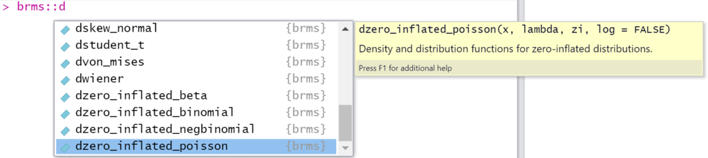
また,様々な確率分布からの乱数を生成するための関数や...

確率(密度)を返す関数も用意されています.
その3
「内部で何をやっているのか」を知ることができます.
ベイズを用いる際に最も気になることの一つが,事前分布の設定でしょう.brmsでは,brms::get_prior()で指定したモデルの事前分布を知ることができます.brmsがデフォルトで採用している事前分布も分かるので,報告時に困ることはありません.
また,brms::make_stancode()で指定したモデルのStanコードを出力させることもできます(公式Vignette).「この確率分布を使ったモデルをStanで書きたいとき,どうすればいいんだろう」と悩んだとき,brmsで同じ確率分布を使った適当なモデルでStanコードを出力させて,「なるほど,こう書けばいいのか」とヒントを得ることも可能です.ちなみにbrms::stancode()はエイリアス(別名)なので,どちらの関数を使っても構いません.
とはいえ,brmsはサンプリング効率を高めるために色々と書き方を工夫しているので,初学者にとって理解しやすいとは限りません.例えばbrms::make_stancode()の公式Vignetteを見てみましょう.これはいわゆる線形混合モデル(ランダム切片モデル)を表していますが,参考書(例:『StanとRでベイズ統計モデリング』)でよく紹介されるモデルとは異なっています.参考書ではよく,次のように紹介されます.
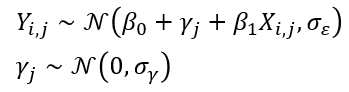
※はてなブログで数式を表示させるのが難しくて,もう数式を画像で貼ることにしました...
しかしbrmsのStanコードは,この数式をそのまま翻訳したようにはなっていませんね(確率分布の違いはこのセクションで言いたいことの本質ではないので無視してください).transformed parametersブロック内でr_1_1 = (sd_1[1] * (z_1[1]));という再パラメータ化を行っていることに注目すると,この謎が解けます.これは,標準正規分布から変量効果をサンプリングしたあとで,変量効果の標準偏差を掛ける,という再パラメータ化を意味します.
※このあたりは,関西学院大学 清水裕士先生より教えていただきました.ありがとうございます.
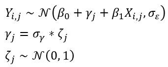
なぜこれによりサンプリングが効率化されるかというと,Stanが実装しているNUTアルゴリズムでは,-2~+2あたりのサンプリングが安定する(らしい)ため,なるべく各パラメータがこの区間から(例えば標準正規分布から)サンプリングされると嬉しいという事情があります.ここで,もともとのモデルではが別のパラメータ
に依存しているため,
がサンプリングされる正規分布自体が揺らぎます.
それに対して再パラメータ化したモデルでは,が他のパラメータに依存せず標準正規分布に従うので,だいたいどのあたりの値がサンプリングされるかが安定するということですね.そこに掛け算される
もまた別のパラメータに依存していないことがポイントです.
その4
他のパッケージとの連携が充実しています.
例えばbrmsはbayesplotパッケージを利用して,brms::pp_check()という関数により,容易に事後予測チェック**を行うことができます(詳しくはこちら).
その他にも,bridgesamplingパッケージを利用してベイズファクターを容易に計算できたり,欠測値がある場合にmiceパッケージで多重代入法による補完を行ったあとで,補完したそれぞれのデータセットからサンプリングを行えたりします(詳しくはこちらから).
brmsパッケージの使用例
それではさっそく使用例を紹介していきましょう.
インストール & ロード
公式VignetteのHow do I install brms?に記載されているように,brmsはCRANから容易にインストール可能です.
ただしその前に,使用予定のRのバージョンに応じて,適切なRtoolsをインストールしておいてください. URLも,上記のVignetteに書いてある通りです.
※例えば,Rバージョン4.4.2を使用するつもりなら,Rtools4.4をインストールする,という具合です.
その後,いつものコマンドを実行すればbrmsが使用できるようになるはずです.
install.packages("brms")
library(brms)
なおbrmsは様々なパッケージと依存関係にあるので,上述のbayesplotパッケージやbridgesamplingパッケージ,それからStanをRから扱うためのrstanパッケージを含む,種々のパッケージが一緒にインストールされます。依存パッケージ一覧は,次のコードで確認できます.
tools::package_dependencies("brms", recursive = TRUE) |> knitr::kable()
# 依存パッケージ数が多いため,knitr::kable()で全行を表示させている
注意
brmsは,バックエンドにrstanとcmdstanrを利用できます(デフォルトはrstan).もしcmdstanrを利用したい場合には,後述するように引数で容易に設定を変えられます.ただし,上記のコマンドを実行するとわかるように,cmdstanrは依存パッケージに含まれていないので,別途インストールしなければいけません.
cmdstanrそのものの説明やインストール方法などは,次のページを参照してください.
一般線形モデル(回帰分析)
まずはベーシックな回帰分析をやってみましょう.プリインストールされている,32台の車の性能が収められたデータセットmtcarsを使用します.
head(mtcars)

                   mpg cyl disp  hp drat    wt  qsec vs am gear carb
Mazda RX4         21.0   6  160 110 3.90 2.620 16.46  0  1    4    4
Mazda RX4 Wag     21.0   6  160 110 3.90 2.875 17.02  0  1    4    4
Datsun 710        22.8   4  108  93 3.85 2.320 18.61  1  1    4    1
Hornet 4 Drive    21.4   6  258 110 3.08 3.215 19.44  1  0    3    1
Hornet Sportabout 18.7   8  360 175 3.15 3.440 17.02  0  0    3    2
Valiant           18.1   6  225 105 2.76 3.460 20.22  1  0    3    1
モデルの指定とサンプリングの実行
燃費(mpg)を,車体重量(wt)とマニュアル車かオートマ車か(am)で予測する重回帰分析を試みます.mtcars$amには0か1が格納されていますが,今回はこれらをfactor型に変換したうえで,交互作用項を含むモデルを指定することにします.
mtcars$am <- as.factor(mtcars$am)
stats::lm()を用いると以下のように書きますが...
fit <- lm(mpg ~ wt * am, data = mtcars)
summary(fit)
brmsでは,どのようなモデルであっても,統一的にbrm()という関数のなかでモデルを指定します.もちろん,rstan::sampling()でサンプリングする際に指定するような諸々の引数も,brm()は対応しています.例えばサンプリング回数(iter),ウォームアップ期間(warmup),乱数のシード(seed),チェイン数(chain),並列化させたいコア数(cores)など.引数は非常に多いので,詳細はコンソール上で?brms::brmと入力してhelpを確認してみてください.
fit <- brm(mpg ~ wt * am,
           data = mtcars,
           iter = 2000,
           warmup = 1000,
           seed = 1234,
           chain = 4,
           cores = 4 # 使用するPCの性能に応じて調整
)
サンプリング結果を格納したオブジェクトをsummary()に入れると要約された結果が返されます.
summary(fit)

# 以下,出力 ---------------------------------
 Family: gaussian
  Links: mu = identity
Formula: mpg ~ wt * am
   Data: mtcars (Number of observations: 32)
  Draws: 4 chains, each with iter = 2000; warmup = 1000; thin = 1;
         total post-warmup draws = 4000

Regression Coefficients:
          Estimate Est.Error l-95% CI u-95% CI Rhat Bulk_ESS Tail_ESS
Intercept    31.55      3.19    25.23    37.83 1.00     1885     2339
wt           -3.82      0.83    -5.45    -2.19 1.00     1923     2322
am1          14.67      4.49     5.97    23.54 1.00     1619     1935
wt:am1       -5.23      1.50    -8.24    -2.28 1.00     1707     2229

Further Distributional Parameters:
      Estimate Est.Error l-95% CI u-95% CI Rhat Bulk_ESS Tail_ESS
sigma     2.68      0.36     2.08     3.51 1.00     2568     2498

Draws were sampled using sampling(NUTS). For each parameter, Bulk_ESS
and Tail_ESS are effective sample size measures, and Rhat is the potential
scale reduction factor on split chains (at convergence, Rhat = 1).
ご覧の通り,summary()で返される結果は,主要な情報が整理されたものになっています.もし各パラメータのMCMCサンプルの要約統計量を愚直に確認したければ,posteriorパッケージのposterior::summarize_draws()を使うと便利です.posteriorパッケージは,brmsの依存パッケージなので,すでにインストールされているはずです.
library(posterior)
posterior::summarize_draws(fit)

# 以下,出力 -------------------------
# A tibble: 8 × 10
  variable      mean median     sd    mad     q5    q95  rhat ess_bulk ess_tail
  <chr>        <dbl>  <dbl>  <dbl>  <dbl>  <dbl>  <dbl> <dbl>    <dbl>    <dbl>
1 b_Intercept  31.6   31.6  3.19   3.26    26.4   36.8   1.00    1885.    2339.
2 b_wt         -3.82  -3.83 0.827  0.831   -5.17  -2.48  1.00    1923.    2322.
3 b_am1        14.7   14.7  4.49   4.41     7.35  22.1   1.00    1619.    1935.
4 b_wt:am1     -5.23  -5.22 1.50   1.45    -7.77  -2.79  1.00    1707.    2229.
5 sigma         2.68   2.64 0.362  0.343    2.17   3.34  1.00    2568.    2498.
6 Intercept    20.1   20.1  0.469  0.466   19.3   20.8   1.00    2568.    2457.
7 lprior       -4.86  -4.86 0.0478 0.0431  -4.95  -4.80  1.00    2459.    2327.
8 lp__        -80.4  -80.0  1.65   1.54   -83.5  -78.3   1.00    1557.    2296.
デフォルトでは,MCMCサンプルの90%区間が表示されます(下限がq5,上限がq95).もしこの区間を95%ベイズ信頼区間に変更したいなら,次のように書いてください.
posterior::summarise_draws(
  fit,
  default_summary_measures()[-5], # "mean", "median", "sd", "mad".5つ目の,90%ベイズ信頼区間を返す関数を除いた
  q2.5 = ~quantile2(.x, probs = 0.025),
  q97.5 = ~quantile2(.x, probs = 0.975),
  default_convergence_measures() # "rhat", "ess_bulk", "ess_tail"
)

# 以下,出力 -------------------------
# A tibble: 8 × 10
  variable      mean median     sd    mad   q2.5  q97.5  rhat ess_bulk ess_tail
  <chr>        <dbl>  <dbl>  <dbl>  <dbl>  <dbl>  <dbl> <dbl>    <dbl>    <dbl>
1 b_Intercept  31.6   31.6  3.19   3.26    25.2   37.8   1.00    1885.    2339.
2 b_wt         -3.82  -3.83 0.827  0.831   -5.45  -2.19  1.00    1923.    2322.
3 b_am1        14.7   14.7  4.49   4.41     5.97  23.5   1.00    1619.    1935.
4 b_wt:am1     -5.23  -5.22 1.50   1.45    -8.24  -2.28  1.00    1707.    2229.
5 sigma         2.68   2.64 0.362  0.343    2.08   3.51  1.00    2568.    2498.
6 Intercept    20.1   20.1  0.469  0.466   19.2   21.0   1.00    2568.    2457.
7 lprior       -4.86  -4.86 0.0478 0.0431  -4.98  -4.79  1.00    2459.    2327.
8 lp__        -80.4  -80.0  1.65   1.54   -84.5  -78.1   1.00    1557.    2296.
他にも,サンプリングしたオブジェクトをbrms::waic()やbrms::loo()に入れると,WAICやlooを計算することもできます(内部ではlooパッケージを使用して計算しています).
brms::waic(fit)

Computed from 4000 by 32 log-likelihood matrix.

          Estimate  SE
elpd_waic    -78.8 4.0
p_waic         4.1 1.0
waic         157.6 7.9

4 (12.5%) p_waic estimates greater than 0.4. We recommend trying loo instead.
brms::loo(fit)

Computed from 4000 by 32 log-likelihood matrix.

         Estimate  SE
elpd_loo    -79.0 4.0
p_loo         4.3 1.1
looic       158.0 8.0
------
MCSE of elpd_loo is 0.1.
MCSE and ESS estimates assume MCMC draws (r_eff in [0.5, 0.9]).

All Pareto k estimates are good (k < 0.7).
See help('pareto-k-diagnostic') for details.
事前分布の表示
brmsは,いくつかのパラメータについてデフォルトで弱情報の事前分布を与えています.今回指定したモデルで,各パラメータにどのような事前分布が与えられていたのかを知るには,brms::get_prior()を使用します.この中にモデルを指定すると,以下のように一覧が表示されます.
brms::get_prior(mpg ~ wt * am, data = mtcars)

                   prior     class   coef group resp dpar nlpar lb ub       source
                  (flat)         b                                         default
                  (flat)         b    am1                             (vectorized)
                  (flat)         b     wt                             (vectorized)
                  (flat)         b wt:am1                             (vectorized)
 student_t(3, 19.2, 5.4) Intercept                                         default
    student_t(3, 0, 5.4)     sigma                               0         default
またbrmsでは基本的に(おそらく常に?),回帰係数bには事前分布は明示されません.つまりデフォルトでは,無情報事前分布が適用されるということになります.これは後述するベイズファクターの計算においては問題となるため,そのような場合にはユーザが事前分布を指定する必要があります.
ところで,上で出力させた事前分布の数値に注目してみてください.例えば切片Interceptのstudent_t(3, 19.2, 5.4)は,値があまりに中途半端で,根拠が気になりますね.
ここで試しに,
- 目的変数を中心化
- 目的変数を標準化
して,デフォルトで指定される事前分布を比較してみましょう.
# 目的変数を中心化.平均が0になるが,標準偏差は変わらない
make_stancode(mpg_c ~ wt * am,
              data = mtcars |>
                dplyr::mutate(mpg_c = mpg - mean(mpg)))

# 以下,出力の一部 -------------
transformed parameters {
  // prior contributions to the log posterior
  real lprior = 0;
  lprior += student_t_lpdf(Intercept | 3, -0.9, 5.4);
  lprior += student_t_lpdf(sigma | 3, 0, 5.4)
    - 1 * student_t_lccdf(0 | 3, 0, 5.4);
}
# 目的変数を標準化.平均が0に,標準偏差が1になる
make_stancode(mpg_z ~ wt * am,
              data = mtcars |>
                dplyr::mutate(mpg_z = (mpg - mean(mpg)) / sd(mpg)))

# 以下,出力の一部 -------------
transformed parameters {
  // prior contributions to the log posterior
  real lprior = 0;
  lprior += student_t_lpdf(Intercept | 3, -0.1, 2.5);
  lprior += student_t_lpdf(sigma | 3, 0, 2.5)
    - 1 * student_t_lccdf(0 | 3, 0, 2.5);
}
事前分布が変わりましたね.まだ調査不足なのですが,恐らく切片の事前分布であるt分布のlocation parameterは,目的変数の平均と標準偏差の情報を使って決められているのではないかと思います.また標準化した際にscale parameterが2.5になるのは,Gelmanによるrstanarmパッケージの仕様を引き継いでいるのではないかと思われます.おそらく回帰係数にも同様に標準偏差の情報を使っているのではないかと思います.
brmsは,なるべくサンプリング結果に対する影響を小さく抑えたうえで弱情報の事前分布を指定している,ということは作者自身が明言していますが,データの情報を使うことが気になるユーザは,次に解説するset_prior()で任意の事前分布を指定するとよいでしょう.
事前分布の指定
ユーザが任意の事前分布を指定したければ,brms::brm()のなかでprior =という引数にパラメータと事前分布をセットで指定します.指定方法には複数の記法があります.詳しくはset_prior()のVignetteを読んでみてください.
fit2 <- brm(mpg ~ wt * am,
            data = mtcars,
            iter = 2000,
            warmup = 1000,
            seed = 1234,
            chain = 4,
            cores = 4,
            prior = c(prior_string("normal(0, 10)", class = "b"),
                      prior(student_t(3, 0, 10), class = Intercept),
                      prior_(~student_t(3, 0, 10), class = ~sigma)
                      )
            )
Stanコードの表示
前述のように,brms::make_stancode()に任意のモデルを指定すると,そのStanコードをコンソールに表示してくれます.例えば先ほど事前分布を指定した,以下のモデルのStanコードを表示してみましょう.長いので,ここではparametersブロック,transformed parametersブロック,modelブロックだけ掲載します.
ちゃんと,ユーザが指定した事前分布も反映されていますね(transformed parametersブロック内の,lprior += normal_lpdf(b | 0, 10);という部分).
brms::make_stancode(mpg ~ wt * am,
                    data = mtcars,
                    prior = c(prior_string("normal(0, 10)", class = "b"),
                              prior(student_t(3, 0, 10), class = Intercept),
                              prior_(~student_t(3, 0, 10), class = ~sigma)
                              )
                    )

# 以下、出力 --------------------------------------------
parameters {
  vector[Kc] b;  // regression coefficients
  real Intercept;  // temporary intercept for centered predictors
  real<lower=0> sigma;  // dispersion parameter
}
transformed parameters {
  real lprior = 0;  // prior contributions to the log posterior
  lprior += normal_lpdf(b | 0, 10);
  lprior += student_t_lpdf(Intercept | 3, 0, 10);
  lprior += student_t_lpdf(sigma | 3, 0, 10)
    - 1 * student_t_lccdf(0 | 3, 0, 10);
}
model {
  // likelihood including constants
  if (!prior_only) {
    target += normal_id_glm_lpdf(Y | Xc, Intercept, b, sigma);
  }
  // priors including constants
  target += lprior;
}
そうそう,brmsのStanコードは全て,target +=記法を用いて書かれています.周辺尤度を計算したり,高度なモデル(例:混合分布モデル)を使ったりする際のことを考えると,最初からtarget記法で書いてくれるのはありがたいですね.
さて,上のコードを見ていただくと,ここでも再び「参考書の書き方と違う!!」と思いませんか.例えば,公式ドキュメントStan User's GuideのRegression Modelsのページを見ていただくと,次のようなStanコードが紹介されています.
data {
  int<lower=0> N;   // number of data items
  int<lower=0> K;   // number of predictors
  matrix[N, K] x;   // predictor matrix
  vector[N] y;      // outcome vector
}
parameters {
  real alpha;           // intercept
  vector[K] beta;       // coefficients for predictors
  real<lower=0> sigma;  // error scale
}
model {
  for (n in 1:N) {
    y[n] ~ normal(x[n] * beta, sigma);
  }
}
じゃあbrmsが吐き出したコードのnormal_id_glm_lpdf()ってなんやねん,って思いますよね.これはStanが用意している,線形回帰分析専用の関数です(公式マニュアル参照).やっていることは,上のy[n] ~ normal(x[n] * beta, sigma);という書き方とほとんど同じです.
このようにbrmsでは,積極的に(Stan User's Guideを読み込まないと知らないような)便利な関数を使ったり,独自にモデルを工夫したりしています.
結果の可視化
plot()
brmsは,サンプリング結果の視覚化にも長けています.rstan::stan_trace()やrstan::stan_dens()のように,描きたいグラフに応じて個別の関数が用意されていることが多いと思いますが,brmsはbayesplotパッケージのbayesplot::mcmc_combo()を用いて結果を可視化します.bayesplotパッケージについては,Stan Advent Calendar 2018の2日目の記事や,11日目の記事をご覧ください.これはbrmsの依存パッケージなので,すでにインストールされているはずです.
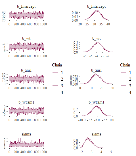
bayesplot::mcmc_combo()は,各パラメータについて,事後分布とトレースプロットを並べて表示してくれます.
※2018年の記事を執筆した時点では,plot()で表示されるmcmc_combo()の結果は,左半分が事後分布のdensity plot,右側がトレースプロットだったのですが,2026年時点では,左側がMCMCサンプルのヒストグラムになっています.
plot(fit)
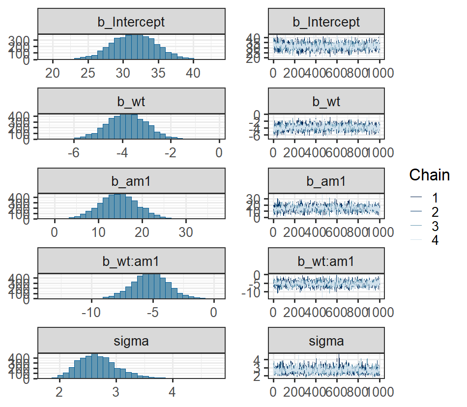
繰り返しますがこのグラフはbayesplotパッケージを用いて出力されているので、同パッケージの関数を用いて見栄え(Aesthetic)を調整することができます。また、bayesplot::mcmc_combo()と同様に、bayesplotパッケージのmcmc_ シリーズの関数のうち、どの種類の関数を組み合わせて表示するかも選択することができます(mcmc_シリーズについては、Stan Advent Calendar 2018 2日目の記事を参照してください)。ただしmcmc_combo()で表示できるグラフの種類は限られているようです。
例えばこんな風に、色調をピンクに変更し、トレースプロット(bayesplot::mcmc_trace())とチェインごとの事後分布(bayesplot::mcmc_dens_overlay())を並べることもできます。
bayesplot::color_scheme_set("pink")
plot(fit, combo = c("trace", "dens_overlay"))
conditional_effects()
さらにbrms::conditional_effects()を用いると、「主効果」や「交互作用」を可視化することもできます。今回は交互作用項を含むモデルを指定したので、いわゆる「単純傾斜」も自動的に可視化されます。下のグラフは、左から順に「wtの主効果」「amの主効果」「wtとamの交互作用」を示します。
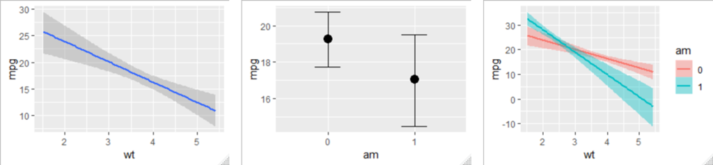
引数effectsに何も指定しなければ、すべての項について可視化が行われますが、特定の項だけを指定することも可能です。また、交互作用項を指定する場合には、その順番を変えることで、どちらの変数についての単純効果を可視化するかも決めることができます。
conditional_effects(fit, effects = "wt:am") #左のグラフ
conditional_effects(fit, effects = "am:wt") #右のグラフ
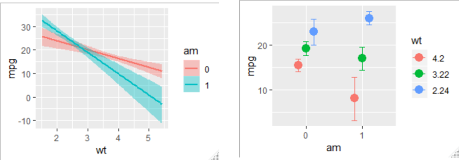
離散変数の場合は(今回はam)、各水準における他方の変数の単純効果が可視化されます。連続変数の場合は(今回はwt)、平均±1SDのポイントにおける、他方の変数の単純効果が示されます。
mean(mtcars$wt) + sd(mtcars$wt) #平均+1SD
[1] 4.195707

mean(mtcars$wt) #平均
[1] 3.21725

mean(mtcars$wt) - sd(mtcars$wt) #平均-1SD
[1] 2.238793
単純効果
交互作用項を含む回帰モデルを実行した場合,単純効果の不確実性を評価したい,すなわち単純効果の事後分布を求めたいことがあります.これには,外部パッケージを使うことを含めると,複数の方法が存在します.ここではbrmsの関数である,brms::hypothesis()を使ってみましょう.
今回のモデルは次の通りでした(添え字は省略しています).と
が各説明変数の主効果,
が交互作用効果を表しています.
この式を変形すると次のようになります.このときが,説明変数
の単純主効果となります.
仮に今回は各説明変数が次の通りだとしましょう.
: 車体重量
wt: オートマ車かマニュアル車か
am- 0(オートマ車),1(マニュアル車)の2値変数
するとオートマ車のとき,の単純主効果は,
となります.交互作用項を含むモデルでダミーコーディングを使う場合,
はいわゆる主効果ではなく,単純主効果であることに注意してください.
同様にマニュアル車のとき,の単純主効果は,
となります.
あとはこの効果についての仮説を検証すればよいのです.brms::hypothesis()はSavage-Dickey法を用いたベイズファクターにより,パラメータについて点で仮説を評価できます(参考).
amがオートマ車のときの,wtの単純主効果が0という仮説は次のように検証します.なおamを因子型に変換した関係で,brms()を実行したときに説明変数の名前がam1に変わったため(summary()の結果を確認してください),am1という変数名を採用しています(もし因子型に変換しなければ,amのままで問題ありません).この数値の1は,単純主効果そのものとは無関係なことに注意してください.
brms::hypothesis(fit, "wt = 0")

# 以下,出力 -----------------------
Hypothesis Tests for class b:
  Hypothesis Estimate Est.Error CI.Lower CI.Upper Evid.Ratio Post.Prob Star
1   (wt) = 0    -3.82      0.83    -5.45    -2.19         NA        NA    *
---
'CI': 90%-CI for one-sided and 95%-CI for two-sided hypotheses.
'*': For one-sided hypotheses, the posterior probability exceeds 95%;
for two-sided hypotheses, the value tested against lies outside the 95%-CI.
Posterior probabilities of point hypotheses assume equal prior probabilities.
点仮説(例えば今回のように,「単純効果が0」)の場合,Evid.Ratioという項目がベイズファクターに相当します.ではベイズファクターがNAとはどういうことでしょうか.
もしこのような結果が表示されたら,brms::hypothesis()のVignetteに書いてあるように,ベイズファクターを計算するうえで重要な設定が抜けているというサインです.後述するように,ベイズファクターを使う関係上,大きなMCMCサンプル数や,無情報でない事前分布などの設定が必要となります(いずれもすでに紹介した引数で容易に設定できます). 詳しくは後ほど改めて詳述するので,ここでは天下り的に,次の通りコードを実行しなおしてみましょう.
# 無情報でない事前分布 -----------------
priors <- c(set_prior("normal(0,5)", class = "b"),
            set_prior("normal(0,5)", class = "Intercept"),
            set_prior("normal(0,5)", class = "sigma")
            )

fit <- brm(mpg ~ wt * am,
           data = mtcars,
           iter = 20000, # サンプリング回数を大きくした
           warmup = 2000,
           seed = 1234,
           chain = 4,
           cores = 4,
           save_pars = save_pars(all = TRUE),
           sample_prior = "yes", # ここが重要!!
           prior = priors # 無情報でない事前分布の指定
)

brms::hypothesis(fit, "wt = 0")

# 以下,出力 -----------------------
Hypothesis Tests for class b:
  Hypothesis Estimate Est.Error CI.Lower CI.Upper Evid.Ratio Post.Prob Star
1   (wt) = 0    -4.59      0.75    -6.09    -3.14          0         0    *
---
'CI': 90%-CI for one-sided and 95%-CI for two-sided hypotheses.
'*': For one-sided hypotheses, the posterior probability exceeds 95%;
for two-sided hypotheses, the value tested against lies outside the 95%-CI.
Posterior probabilities of point hypotheses assume equal prior probabilities.
Evid.Ratioが正しく数値で表示されました.単純効果が0という仮説の対立仮説に対するBayes factorが0(厳密に0というより,ほとんど0という意味)ということは,単純効果は0でないという仮説のほうがデータと整合的ということです.
同様にamがマニュアル車のときの,wtの単純主効果が0という仮説の検証方法は,次の通りです.brms::conditional_effects()が出力したグラフから明らかなように,オートマ車でもマニュアル車でも,車体重量wtが大きくなるほど燃費mpgが悪くなることは変わらないようです.
brms::hypothesis(fit, "wt + wt:am1  = 0")

# 以下,出力 -----------------------
Hypothesis Tests for class b:
       Hypothesis Estimate Est.Error CI.Lower CI.Upper Evid.Ratio Post.Prob Star
1 (wt+wt:am1) = 0    -7.59      1.16     -9.8    -5.22          0         0    *
---
'CI': 90%-CI for one-sided and 95%-CI for two-sided hypotheses.
'*': For one-sided hypotheses, the posterior probability exceeds 95%;
for two-sided hypotheses, the value tested against lies outside the 95%-CI.
Posterior probabilities of point hypotheses assume equal prior probabilities.
さて,brms::hypothesis()の実行結果をみると,ベイズファクター以外にも様々な数値が出力されています.これらは,帰無仮説検定で単純効果が「有意かどうか」を調べる伝統的な方法に相当します.帰無仮説検定の文脈では,単純効果の95%信頼区間の下限CI.Lowerと上限CI.Upperが0をまたいでいなければ,「有意な効果がある」と判断するのでした.ベイズ信頼区間を用いて同様の推測を行うことは可能です.ただしbrmsの作者は,安易に恣意的な基準で効果の有無を論じることには警鐘を鳴らしています.
この事後期待値(Estimate)や,事後標準誤差(Est.Error),95%ベイズ信頼区間(CI.Lower, CI.Upper)を検算してみましょう.MCMCによるパラメータ推定の便利なところは,MCMCサンプルを引っこ抜けば任意の計算が可能なことです.
データフレームでMCMCサンプルを抜くには,brms::as_draws_df()を使います.
s <- brms::as_draws_df(fit)
head(s)

# 以下,出力 ---------------------
# A draws_df: 6 iterations, 1 chains, and 8 variables
  b_Intercept b_wt b_am1 b_wt:am1 sigma Intercept lprior lp__
1          30 -3.0    12     -4.5   2.5        21   -4.9  -81
2          36 -4.6    10     -4.8   3.3        21   -5.0  -83
3          39 -5.3     9     -4.7   3.3        21   -5.0  -84
4          29 -3.1    16     -5.3   2.6        20   -4.8  -78
5          29 -3.2    17     -5.7   2.7        20   -4.9  -78
6          30 -3.3    15     -5.3   2.6        21   -4.9  -79
# ... hidden reserved variables {'.chain', '.iteration', '.draw'}
amがオートマ車のときの,wtの単純主効果を計算してみましょう.確かに,brms::hypothesis()の結果と一致しています.
mean(s$b_wt + s$`b_wt:am1`) # 事後期待値
# [1] -9.05513

sd(s$b_wt + s$`b_wt:am1`) # 事後標準誤差
# [1] 1.253566

quantile(s$b_wt + s$`b_wt:am1`, c(0.025, 0.975)) # 95%ベイズ信頼区間
#       2.5%      97.5%
# -11.586738  -6.657283
事後予測チェック
事後予測チェックについては,Stan Advent Calendar 2018 11日目の記事も参照してください.Stanでモデルを書いた場合,事後予測チェックを行うためには,generated quantitiesブロックでモデルから乱数を生成させる手続きが必要になります.その乱数を抽出して,実際に観測されたデータとの類似性を把握するわけですが,brmsではサンプリング結果が格納されたオブジェクトをbrms::pp_check()に入れるだけで,事後予測チェックができます.
brms::pp_check(fit)
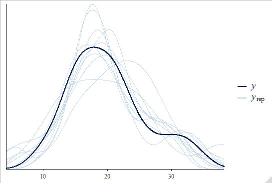
Stan Advent Calendar 2018 11日目の記事を読んだ方はお察しの通り,これは内部でbayesplot::ppc_dens_overlay()を使用しています.
他の事後予測チェックにも対応しています.type =という引数に,描画形式を指定してみます.
brms::pp_check(fit, type = "error_hist")
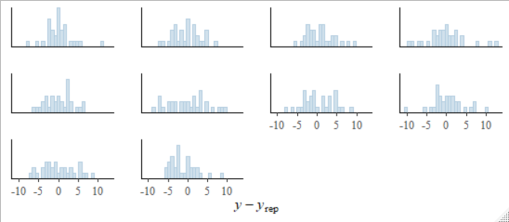
これはbayesplot::ppc_error_hist()を使用していますね.
一般化線形モデル
次は,正規分布以外の指数分布族を扱えるように拡張した,一般化線形モデルを例に挙げます.今度は目的変数を,オートマ車かマニュアル車かamにし,説明変数に燃費mpgと重量wtを投入してみます.
stats::glm()と同様に,目的変数が従う確率分布を,引数family =に指定しましょう.今回は,オートマ車かマニュアル車かamは2値の変数なので,family = "bernoulli"とベルヌーイ分布を指定します(余談ですが,stats::glm()では2値の目的変数に対しては二項分布(family = "binomial")を指定しますが,brmsでは2値の目的変数に対して二項分布を指定すると,Only 2 levels detected so that family 'bernoulli' might be a more efficient choice.とサジェストされます).
ただしbrmsでは,family = "binomial"を指定した際の記法がstats::glm()と異なるので,ここでは紹介のためあえて二項分布を適用した書き方をしてみます.
stats::glm()ではこのように書きます.
#amをfactor型に変換していたのを,いったんリセット
data(mtcars)

fit <- glm(cbind(am, 1 - am) ~ mpg + wt,
           family = "binomial",
           data = mtcars)
#目的変数が2値の場合は、
#fit <- glm(am ~ mpg + wt, family = "binomial", data = mtcars) でOK

summary(fit)
cbind()のなかで何をしているのかというと,総試行数中に占める,成功試行数(am)と失敗試行数(1 - am)の列を指定しています.今回は1台の車がオートマ車かマニュアル車かを予測するので,試行数は1であるため,失敗試行の列は1 - amとしています.
さてbrmsでは,目的変数が二項分布に従うと仮定するとき,以下のように書きます.|の左側には成功試行数を,右側にはtrials()の中に試行数を入れます.
#amをfactor型に変換していたのを,いったんリセット
data(mtcars)

fit <- brm(am | trials(1) ~ mpg + wt,
           family = "binomial",
           data = mtcars)
#目的変数が2値の場合は、
#fit <- brm(am ~ mpg + wt, family = "bernoulli", data = mtcars) でOK

summary(fit)
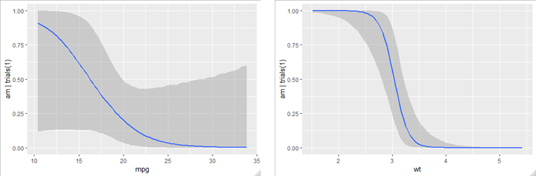
brms::conditional_effects()で主効果を可視化してみると,ロジットリンク関数によって、直線ではなく曲線になっていることがわかりますね.
豊富なbrms family
ゼロ過剰ポアソン分布
さて,ここからがbrmsの真骨頂です.stats::glm()ではfamilyに指定できる確率分布は以下の通りです.
- gaussian
- binomial
- Gamma
- inverse.gaussian
- poisson
- quasi
が,brmsでは豊富なfamilyが用意されているということを冒頭で述べました.試しにちょっと珍しい分布を使ってみましょう.
皆さんは,先月,何回観劇しましたか? ちなみに私は3回です.今月も3回行く予定です.
恐らく0回か,多くとも1回と回答する人が多いのではないでしょうか.ヒストグラムを描くと,次のようになったと仮定します.
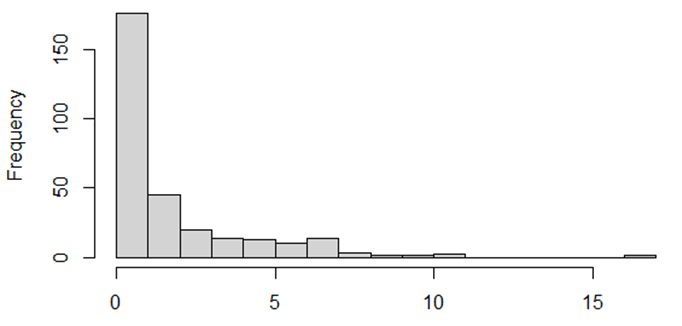
さて,観劇回数はカウントデータなので,ポアソン分布と相性がよさそうに思えますが,上図のとおり0が圧倒的に多く,通常のポアソン分布の仮定を満たしそうにありません.そこで,0が通常のポアソン分布よりも過剰であるという特徴を捉えた,ゼロ過剰ポアソン分布(zero-inflated poisson)という確率分布を考えます.
ゼロ過剰ポアソン分布は,ベルヌーイ分布とポアソン分布の混合分布です.観劇ファンか否かがベルヌーイ分布に従うとと考え,もし興味がないなら当然観劇回数は0.もし興味があるなら,観劇数はポアソン分布に従う,と考えます.ポアソン分布に従う確率変数は0以上の整数をとるので,観測された「0回」というデータの背後には,
- ベルヌーイ分布から生成された0
- ポアソン分布から生成された0
の二つが混在していると仮定します.

さて,ここでは架空の例として,観劇ファンは,自宅から最寄りの劇場までの所要時間が短いほど,観劇回数が多いというシナリオを考えてみましょう.まずはこの仮定を満たすサンプルデータを生成してみます.
set.seed(123)
n <- 300 # 総サンプルサイズ
minute <- rnorm(n, mean = 40, sd = 10) # 説明変数(所要時間)
lambda <- exp(4 - 0.08 * minute) # 切片と回帰係数の真値を設定
theta <- 0.3 # 観劇ファンである確率
zeros <- rbinom(n, size = 1, prob = theta) # 0 or 1の乱数を生成
num <- ifelse(zeros == 1, 0, rpois(n, lambda)) # 観劇ファンならポアソン分布から乱数を生成,非ファンなら0

par(mfrow = c(1, 2)) # 可視化の設定
hist(num, breaks = 15) # 鑑賞回数のヒストグラム
plot(minute, num) # 所要時間と鑑賞回数の散布図
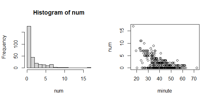
次に,月の観劇回数がゼロ過剰ポアソン分布に従うと仮定し,最寄りの劇場までの所要時間で予測するモデルを推定してみましょう.Stanでモデルを書くとしたら,Stan User's Manualにあるように、target +=という記法を用いたり,log_sum_exp()関数を使ったりして,少し工夫した書き方が必要になります.
しかしbrmsではfamily = "zero_inflated_poisson"を指定するだけで推定できます.なお分布名だけを指定すると,ポアソン分布のパラメータに対して回帰するモデルが適用されます.
fit_zip <- brm(num ~ minute,
           data = data.frame(num, minute),
           family = "zero_inflated_poisson",
           seed = 1234)

summary(fit_zip)

# 以下,出力 ----------------------------
 Family: zero_inflated_poisson
  Links: mu = log
Formula: num ~ minute
   Data: data.frame(num, minute) (Number of observations: 300)
  Draws: 4 chains, each with iter = 2000; warmup = 1000; thin = 1;
         total post-warmup draws = 4000

Regression Coefficients:
          Estimate Est.Error l-95% CI u-95% CI Rhat Bulk_ESS Tail_ESS
Intercept     4.01      0.19     3.66     4.36 1.00     3110     2872
minute       -0.08      0.01    -0.09    -0.07 1.00     2576     2570

Further Distributional Parameters:
   Estimate Est.Error l-95% CI u-95% CI Rhat Bulk_ESS Tail_ESS
zi     0.30      0.03     0.23     0.36 1.00     2361     2280

Draws were sampled using sampling(NUTS). For each parameter, Bulk_ESS
and Tail_ESS are effective sample size measures, and Rhat is the potential
scale reduction factor on split chains (at convergence, Rhat = 1).
びっくりするほど綺麗に,パラメータリカバリできていますね....
事後予測チェックしてみましょう.
brms::pp_check(fit_zip)
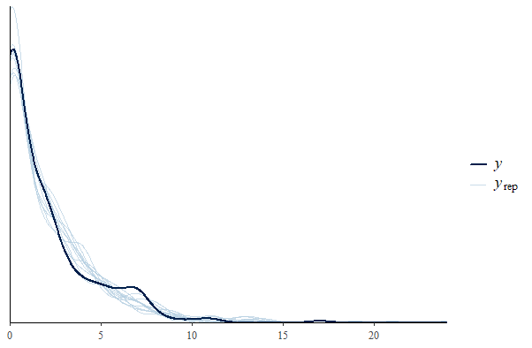
いい感じですね.
今回推定したモデルは,真のデータ生成メカニズム(サンプルデータを生成した際のアルゴリズム)を正しくとらえているので,リカバリに成功したのはある意味で当然といえます.実際の研究では真のデータ生成メカニズムは不明なので,モデルが乖離する可能性があります.
試しに,ポアソン分布のパラメータだけでなく,ベルヌーイ分布のパラメータ
に対しても同時に予測を試みてみましょう.このような複雑なモデルすらも,柔軟に表現できるのが
brmsの凄いところです.柔軟にモデルを書くためには,brms::bf()という関数を使います(bfは,brmsformulaの略です.詳しくはVignetteを参照).
brmsが用意しているゼロ過剰ポアソン分布(brms::zero_inflated_poisson())をfamilyに指定する場合,ベルヌーイ分布のパラメータはziという名前になっています.上の,summary(fit_zip)の出力結果に,Further Distributional Parameters: ziと書かれていることに注目してください.そのため,ziを説明変数minuteで回帰するモデルを追記すればよいのです.
fit_zip2 <- brm(brms::bf(num ~ minute, zi ~ minute),
                data = data.frame(num, minute),
                family = "zero_inflated_poisson",
                seed = 1234)

summary(fit_zip2)

# 以下,出力 -----------------------
 Family: zero_inflated_poisson
  Links: mu = log; zi = logit
Formula: num ~ minute
         zi ~ minute
   Data: data.frame(num, minute) (Number of observations: 300)
  Draws: 4 chains, each with iter = 2000; warmup = 1000; thin = 1;
         total post-warmup draws = 4000

Regression Coefficients:
             Estimate Est.Error l-95% CI u-95% CI Rhat Bulk_ESS Tail_ESS
Intercept        4.05      0.19     3.67     4.41 1.00     2600     3025
zi_Intercept    -0.41      0.81    -1.97     1.22 1.00     2397     2665
minute          -0.08      0.01    -0.09    -0.07 1.00     2219     2575
zi_minute       -0.01      0.02    -0.06     0.03 1.00     2086     2205

Draws were sampled using sampling(NUTS). For each parameter, Bulk_ESS
and Tail_ESS are effective sample size measures, and Rhat is the potential
scale reduction factor on split chains (at convergence, Rhat = 1).
階層線形モデル
本記事冒頭でも言及したように,lme4パッケージやlmerTestパッケ―ジを用いると,以下のように書きますよね.
lme4::lmer(y ~ x + (1 | group), data = dat)lme4::glmer(y ~ x + (1 | group), family = "poisson", data = dat)
brmsでは,関数をbrm()に変えるだけで同じように階層線形モデルを推定できます.
ただし,ベイズモデリングの強みは柔軟なモデルを表現・推定できることですから,最尤法では推定できなかったような複雑なモデルも表現できます.やや高度な話になるので詳述はしませんが,詳しくは以下のリンクからAdvanced Multilevel Modeling with brmsを参照してください.このページにはそのほかにも高度な書き方を要する情報が掲載されています.
モデル比較
brmsパッケージを用いてサンプリングした結果を利用して,モデル比較を行ってみます.モデル比較には様々な観点がありますが,ここではベイズファクターを指標とすることにします.ベイズファクターについては北條大樹さんのこちらの記事や,清水裕士さんのスライドをご参照ください.
brmsを用いてモデル比較するために,kidneyというデータセットを用いて試してみましょう.survivalパッケージにも同じ名前のデータセットがあるので,区別するためにbrms::kidneyと指定したほうが無難です.
話を簡単にするために,ここでは目的変数に「病気の再発までの時間time」,説明変数に「患者の年齢age」を投入した,単回帰分析を考えます.また,本当は右側打ち切り(right-censored)が起こっているため,それを考慮したモデリングをするべきですが(brmsなら容易に実現できます),打ち切りが起こっていないデータだけを抽出しています.
なおbrmsでは,brm(y | cens(censored) ~ x, data = dat)のように書くことで,打ち切りデータのモデリングも容易に実現できます(cens()のなかに,打ち切りの有無を判別する変数を投入します).
#データセットの作成 ---------------------------------------------
#1回目の再発までの時間 & 非打ち切りデータのみを使用
dat <- brms::kidney %>%
  dplyr::filter(recur == "1" & censored == 0)

#データセットの行列数 -------------------------------------------
dim(dat) #38人分のデータが抽出された
[1] 38  7

#冒頭6行分を表示 ------------------------------------------------
head(dat)

  time censored patient recur age    sex disease
1    8        0       1     1  28   male   other
2   23        0       2     1  48 female      GN
3   22        0       3     1  32   male   other
4  447        0       4     1  31 female   other
5   30        0       5     1  10   male   other
6   24        0       6     1  16 female   other
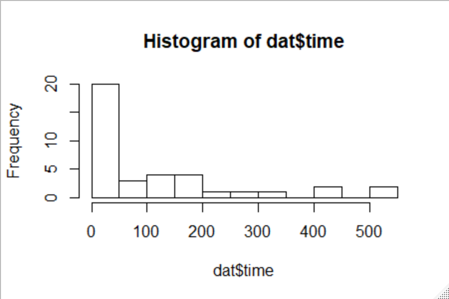
目的変数timeの分布はこのように左に歪んでいます.
正規分布を仮定したモデル
まずはベーシックな単回帰分析を実行してみます.目的変数が正規分布に従うと想定することになるので,family = "normal"と指定します(familyを指定しなければ自動的に正規分布を仮定することになるので、省略も可能です).
さらに以下3点を対処する必要があります.
- 全パラメータに,無情報でない事前分布を指定
iterを多めに- 正確には,有効なMCMCサンプルの数を多めに
save_pars = save_pars(all = TRUE)と引数を指定- ※重要:以前は
save_all_pars = TRUEだったが,変更になった
- ※重要:以前は
sample_prior = "yes"と引数を指定- 重要:事前分布からもサンプリングするため.以前はこの引数はなかったような気がする...
- デフォルトは"no".
- 事前予測チェックが目的なら,事前分布からのみサンプリングするので,"only"にする.
モデルはこのようになります.
fit_n <- brm(time ~ age,
             family = "normal",
             prior = prior(normal(0, 5), class = b),
             seed = 1234,
             iter = 100000,
             warmup = 5000,
             data = dat,
             save_pars = save_pars(all = TRUE),
             sample_prior = "yes"
)
事後予測チェックを行ってみましょう.
brms::pp_check(fit_n)
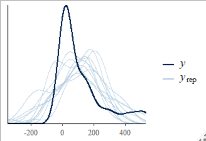
実際に観測されたデータとズレがありますね.上のヒストグラムを見ればわかる通り,今回はtimeが正規分布に従うと仮定するのは適切ではないかもしれません.
最後にbrms::bridge_sampler()を用いて,bridge samplingによる対数周辺尤度を計算してみましょう.これは内部ではbridgesampling::bridge_sampler()を利用しています.
set.seed(123)
bs_n <- brms::bridge_sampler(fit_n)
lml_n <- bs_n$logml # 対数周辺尤度(log marginal likelihood)
bs_n

# 以下,出力 ------------------------
Iteration: 1
Iteration: 2
Iteration: 3
Iteration: 4
Bridge sampling estimate of the log marginal likelihood: -249.9511
Estimate obtained in 4 iteration(s) via method "normal".
ワイブル分布を仮定したモデル
brms::kidneyは生存時間解析に適したデータセットなので,比較対象としてパラメトリックな生存時間解析でよく用いられる,ワイブル分布を適用したモデルを考えてみます.
fit_w <- brm(time ~ age,
             family = weibull(),
             prior = prior(normal(0, 5), class = b),
             seed = 1234,
             iter = 100000,
             warmup = 5000,
             data = dat,
             save_pars = save_pars(all = TRUE),
             sample_prior = "yes"
)
事後予測チェック.
brms::pp_check(fit_w)
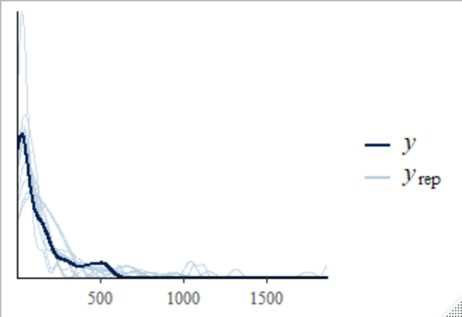
先ほどよりマシになった気がしますね.
次はbridge samplingによる対数周辺尤度の計算.
set.seed(123)
bs_w <- brms::bridge_sampler(fit_w)
lml_w <- bs_w$logml # 対数周辺尤度(log marginal likelihood)
bs_w

# 以下,出力 ------------------------
Iteration: 1
Iteration: 2
Iteration: 3
Iteration: 4
Bridge sampling estimate of the log marginal likelihood: -230.8442
Estimate obtained in 4 iteration(s) via method "normal".
正規分布 vs ワイブル分布
いよいよモデル比較です.各モデルの対数周辺尤度を指数変換して周辺尤度に戻し,比をとるとベイズファクターになります.ただしexp(lml_w) / exp(lml_n)と計算すると(分子のほうが,より仮説に近いモデル),対数周辺尤度次第では,指数変換したときに極めて大きな値となり正確に計算できなくなる恐れがあります.
そこで式変形して,次のように計算したほうが安全です(一つ目のほうが,より仮説に近いモデル).
exp(lml_w - lml_n) #ベイズファクター.より仮説に近いほうのモデルを一つ目にする

[1] 198619204
各モデルの対数周辺尤度を符号反転させて自由エネルギーに変換した場合は,exp()内のモデルの順番が逆なことに注意してください.
fe_n = -1 * lml_n  #正規モデルの自由エネルギー 249.9511
fe_w = -1 * lml_w  #ワイブルモデルの自由エネルギー 230.8442

exp(fe_n - fe_w) #ベイズファクター.より仮説に近いほうのモデルを二つ目にする

[1] 198619204
今回のデータに対する当てはまりの観点では,正規分布を仮定したモデルに対して,ワイブル分布を仮定したモデルを支持する程度が,198619204倍...もう圧倒的に大きいと考えられます.
なおbrmsは,bridgesampling::bayes_factor()を利用して直接ベイズファクターを計算する,brms::bayes_factor()という関数を用意しています.引数x1とx2に,各モデルのサンプリング結果を格納したオブジェクトを指定してください.
set.seed(123)
brms::bayes_factor(x1 = fit_w, x2 = fit_n) # より仮説に近いモデルがx1

# 以下,出力 --------------------
Iteration: 1
Iteration: 2
Iteration: 3
Iteration: 4
Iteration: 1
Iteration: 2
Iteration: 3
Iteration: 4
Estimated Bayes factor in favor of bridge1 over bridge2: 198464340.00701
やはり今回のデータに対する当てはまりの観点では,正規分布を仮定したモデルよりも,ワイブル分布を仮定したモデルのほうが良いと考えられます.
こんな風に,brmsを用いてモデル比較をすることもできます.ただしモデル比較という手続きは非常に難しいので,実際にはもっと慎重に行う必要があると思います.
以下,北條さんの記事から引用します.
ベイズファクターの注意点
- ベイズファクターは事前分布の影響をかなり大きくうけます
- 同一データ,同一モデルで事前分布のみを変化させた場合に,どれだけベイズファクターが変化するかを検討するととてもよくわかります.
bridgesamplingパッケージでも計算がうまく行かないことはありますので,全てのモデル間のベイズファクターが計算できるわけではありません.- モデル比較を行うのはとても難しいです.
- 本来,我々が比較すべきモデルは無限に存在します.
- ベイズファクターは,二つのモデル間の比として考えるので,それ以外のモデルについては考えてはいません.
2019/12/6追記
清水裕士さんによる,Stan Advent Calendar 2019 6日目の記事:brmsパッケージで安易にベイズファクターを使うと死ぬ話で,brmsでベイズファクターを求める際の注意点が書かれています.
その他のtips
関数名の前にbrms::と付けるクセをつける
あくまで個人的な意見ですが,何かしらのパッケージ内の関数を使用する場合には,パッケージ名を併記したほうがいいと思っています(例えばdplyr::select()とか).これはいくつかの理由がありますが,一番の理由は,たまに複数のパッケージ間で同じ名前の関数が存在することがあるからです.例えばfilter()という関数は,少なくともstatsパッケージとdplyrパッケージに存在します.
また,他者とコードを共有するときに,何のパッケージの関数か分からないと混乱を招くと思うので,そういった意味でもパッケージ名を明示しておいた方がいいかなと思っています. もちろん,文字数が増えるのでコードが見にくくなるという側面もありますが.
ただ,brmsパッケージを用いる際には,特に意識してbrms::と書いたほうがよいと思います.これは何故かというと,brmsは様々なパッケージに依存しているのですが,データセット名や関数名が衝突することがあるからです.例えば以下のようなデータセットや関数たち.
brms::kidneyデータセットとsurvival::kidneyデータセットbrms::bayes_factor()とbridgesampling::bayes_factor()brms::bridge_sampler()とbridgesampling::bridge_sampler()brms::bf()とbridgesampling::bf()
一番タチが悪いのが最後のbf()です.bridgesampling::bf()はベイズファクターを計算する関数で,bridgesampling::bayes_factor()のエイリアス(略称)なのですが,brms::bf()はベイズファクターとは関係がありません.brms::bf()は,brms::brmsformula()の略称で,brmsを用いて高度なモデリングを可能にするための関数です.
任意の分位点(例えば,20パーセンタイル点)を予測する,分位点回帰を例に説明します.この場合,asymmetric Laplace分布を適用して,以下のように書きます.前述のように,brm()の中にさらにbf()という関数を書いて,その中でモデルを指定します.
以下のコードでは分位点回帰の仕組みを例示するため,説明変数を投入せず切片だけのモデル(説明変数が1)にしています.
fit_q <- brm(bf(mpg ~ 1, quantile = 0.2),
             data = mtcars,
             family = asym_laplace(),
             seed = 1234
)

summary(fit_q)

# 以下,出力 ----------------------------
 Family: asym_laplace
  Links: mu = identity
Formula: mpg ~ 1
         quantile = 0.2
   Data: mtcars (Number of observations: 32)
  Draws: 4 chains, each with iter = 2000; warmup = 1000; thin = 1;
         total post-warmup draws = 4000

Regression Coefficients:
          Estimate Est.Error l-95% CI u-95% CI Rhat Bulk_ESS Tail_ESS
Intercept    15.13      0.66    13.79    16.45 1.00     2573     1785

Further Distributional Parameters:
         Estimate Est.Error l-95% CI u-95% CI Rhat Bulk_ESS Tail_ESS
sigma        1.51      0.28     1.05     2.15 1.00     2870     2695
quantile     0.20      0.00     0.20     0.20   NA       NA       NA

Draws were sampled using sampling(NUTS). For each parameter, Bulk_ESS
and Tail_ESS are effective sample size measures, and Rhat is the potential
scale reduction factor on split chains (at convergence, Rhat = 1).
mtcarsパッケージの変数mpgは,20パーセンタイル値が15.2なので,確かにほとんど正確に推定できていますね.
quantile(mtcars$mpg, 0.2)

 20%
15.2
ここでもしbridgesampling::bf()のほうが読み込まれてしまうと,当然エラーになります.多分大丈夫じゃないかなと思いますが,不安な人はbrms::bf()とパッケージ名を明記してもいいかもしれません.
あるいは,パッケージの優先順位をつけてもいいかもしれないですね.
参考記事:R でパッケージの優先順位を変えたい #rstatsj
おわりに
ここで紹介した機能は,brmsのほんの一部にすぎません.モデリングの自由度もかなり高いですし,ユーザも多いのでWeb上で色んな情報を得ることができます.
例えばこちらの記事では,brmsを用いて信号検出理論のパラメータを推定しています.
きっとこれからも,どんどん新しい機能が追加されていくと思うので,要チェックですね.
そういえばこの記事を書くためにbrmsについて調べていたら,brmsとggplot2とtidyverseを用いてStatistical Rethinkingを解説**しているドキュメントを見つけました.
Statistical Rethinking with brms, ggplot2, and the tidyverse
あと,brmsの作者自身がbrms bookというプロジェクトで解説ドキュメントを作っていました(この記事を書き終わってから気づいた).鋭意更新中だそうなので,チェックしてみてください.
Enjoy!!
JATOSでオンライン実験を実行した際のデータをRに読み込む方法
記事の目的
心理学におけるオンライン実験のノウハウの備忘録です.
友人に助けていただいて,初めてJATOSを用いてlab.jsで作成した実験を走らせてみました(何の話だ,という人は以下のページなどを参照してください).
JATOS上に保存されたデータは.json形式になっているので,解析のためにRに読み込むためにひと手間が必要です...という知識は知っていたのですが,想像以上に面倒くさかったです.
試行錯誤した結果,恐らく最も楽であろう方法がわかったので,将来の自分のためにメモしておきます.
手順
1. JSONから必要なデータをダウンロードする
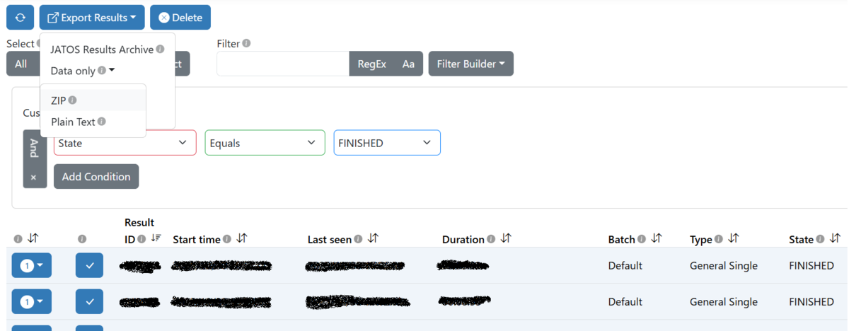
Filter機能を使って最後まで実験を完遂した人のデータ(State == FINISHED)だけを選択したのち,Export Results → Data only → ZIP でデータを一括ダウンロードします.
まずここが面倒くさいポイントで,ZIPファイルを展開すると,参加者ごとに個別のフォルダが作成されていることがわかります.その「参加者ごとのフォルダの中の中」に,データが格納された.jsonファイルがdata.txtという名前で格納されています.
そう,各参加者のフォルダの中には,サブフォルダがあり(しかも名前が違う!),そのさらに中に読み込みたいファイルがあるのです.
補足
ちなみにJATOSからデータをエクスポートするとき,上記のZIPではなく,Plain Textを選ぶこともできます(上図「JATOSのメニュー」で,ZIPの真下にPlain Textの文字が見えます).
本来,こちらをダウンロードすれば,最初から全員分のデータが一つにまとまった.jsonファイルが手に入るはずなのですが,自分の環境では元々のプログラムのせいかわかりませんが,うまくRに読み込めませんでした.そのため上記のようにZIPでダウンロードする方針をとったという経緯があります.
2. サブフォルダの中にある.jsonファイルを読み込む
以前に以下の記事で書いたコードを修正して,今回の問題に挑みます.
library(purrr)
library(jsonlite)

# 自作関数
# read_json(simplifyVector = TRUE)により,読み込んだ.jsonファイルがデータフレームになる
read_func = function(x){jsonlite::read_json(x, simplifyVector = TRUE)}

# 読み込みたい全ファイル名の一括取得
target_files = list.files(path = "hogehoge/", # 展開したZIPファイルの一番上の階層
                          pattern = ".txt$",  # 参加者ごとのデータが格納された.jsonファイルを正規表現で探す
                          recursive = TRUE, # ここが重要.サブフォルダも含めて,条件に合致するファイルを再帰的に探す
                          full.names = TRUE)

# ファイルの結合
dat = purrr::map_df(target_files, read_func) # 各データフレームを,縦方向に結合していく
ポイント①:recursive = TRUE
この引数の存在を知らなかったので,普通に勉強になりました.これにより,サブフォルダ内も探させることができます.
ポイント②:jsonlite::read_json()
最初はこちらのページを参考に,jsonlite::fromJSON()を使おうとしたのですが,自分のケースだと変なところでヘッダ行が折り返されてしまい,綺麗なデータフレームになりませんでした.
他の方法を探したところ,以下の記事で解説されていた,同じくjsonliteパッケージの関数jsonlite::read_json()を見つけました.試したところ,バッチリ綺麗に整形されたデータフレームが手に入りました.simplifyVector = TRUEの引数をお忘れなく.
ggplot2の(正確にはHmiscの)関数が返す区間を、自力で計算した出力と比較する
目的
ggplot2パッケージの関数で、95%信頼区間など、母数の区間推定の実現値を直接可視化できる。 この計算が、自力で計算した値と本当に(ほぼ)一致するか調べる。
参考資料
なお本記事は現時点で執筆中。
mean_cl_normal()
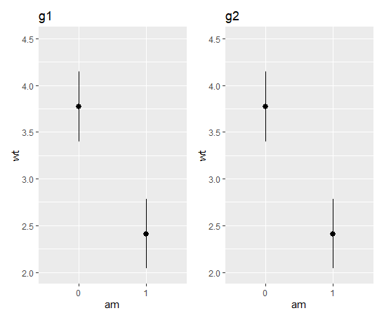
データが正規分布にi.i.d.に従うと仮定できる場合。以下の2通りのコードはどちらも同じ出力を返すはず。
なお以下のコードではmtcars$wtの母平均を推定する文脈で可視化しているが、このデータに関して上記の仮定が満たされるかどうかは今回は考慮していない(コードを示すことが目的なので)。
library(tidyverse)

# ggplotの関数で95%信頼区間を計算した場合 ---------

g1 = ggplot(data = mtcars,
            mapping = aes(x = factor(am), y = wt)) +
  stat_summary(fun.data = "mean_cl_normal") +
  coord_cartesian(ylim = c(2, 4.5)) +
  labs(x = "am", title = "g1")

g1


# 自力で95%信頼区間を計算した場合 ---------
g2 = mtcars %>%
  dplyr::group_by(am) %>%
  dplyr::summarise(mean = mean(wt),
                   upper_cl = mean(wt) +
                     qt(0.975, n() - 1) * (sd(wt) / sqrt(n())),
                   lower_cl = mean(wt) -
                     qt(0.975, n() - 1) * (sd(wt) / sqrt(n()))
  ) %>%
  ggplot(mapping = aes(x = factor(am), y = mean)) +
  geom_pointrange(mapping = aes(ymax = upper_cl, ymin = lower_cl)) +
  coord_cartesian(ylim = c(2, 4.5)) +
  labs(x = "am", y = "wt", title = "g2")

g2
mean_cl_boot()
標本平均を点で、ノンパラメトリック・ブートストラップ法による、ブートストラップ信頼区間をエラーバーで表したグラフ。 ブートストラップ法なので、厳密に一致させることはそもそもできないが、ほぼ同じとみてよい?
library(tidyverse)

# ggplotの関数で95%信頼区間を計算した場合 ---------
g3 = ggplot(data = mtcars,
            mapping = aes(x = factor(am), y = wt)) +
  stat_summary(fun.data = "mean_cl_boot") +
  coord_cartesian(ylim = c(2, 4.5)) +
  labs(x = "am", title = "g3")

g3


# 自力で95%信頼区間を計算した場合 ---------
iter = 3000 # ブートストラップ標本数
m = data.frame(
  a_boot_mean = rep(0, iter),
  m_boot_mean = rep(0, iter)
)

set.seed(123)
for(j in 1:2){
  # ここはややこしいが、am == 0とam == 1があるので
  df = mtcars %>% dplyr::filter(am == (j - 1))
  for(i in 1:iter){
    # dfと同じサイズを復元抽出して、wtの平均を計算
    m[i, j] = dplyr::sample_frac(tbl = df, size = 1, replace = TRUE) %>%
      dplyr::pull(wt) %>%
      mean()
  }
}

g4 = mtcars %>%
  dplyr::group_by(am) %>%
  dplyr::summarise(mean = mean(wt)) %>%
  dplyr::mutate(upper = c(quantile(m[,1], 0.975), quantile(m[,2], 0.975)),
                lower = c(quantile(m[,1], 0.025), quantile(m[,2], 0.025))
                ) %>%
  ggplot(mapping = aes(x = factor(am), y = mean)) +
  geom_pointrange(mapping = aes(ymax = upper, ymin = lower)) +
  coord_cartesian(ylim = c(2, 4.5)) +
  labs(x = "am", y = "wt", title = "g4")

g4

{cowplot}で複数のグラフを結合する / {ggh4x}でX 軸・Y 軸のラベルをうまく扱う
第109回R勉強会@東京(#TokyoR)(データ可視化特集会)でトークしてきました
光栄なことに、応用セッションにご招待いただき、「複数のグラフを1枚のFigureにまとめるとき、cowplotのこと、時々でいいから、思い出してください」というタイトルでトークしてきました。
タイトルにはcowplotしか書いていませんが、実際にはcowplotとggh4xという2つのパッケージの紹介を行いました。
とても勉強になる発表ばかりで、楽しかったです。また機会があれば参加・発表させていただきたいと思います。
Enjoy!
以下、個人的メモ
最後の方で、secondary Y axisの任意の位置に目盛を打ち、文字ラベルを表示させる方法を紹介しています。もし数値目盛を打つのでよければ以下の記事が参考になります(ユタニさんに教えていただきました)。
【新刊案内】『数値シミュレーションで読み解く統計のしくみ 〜Rでためしてわかる心理統計』
書籍の紹介
2023年9月13日に、技術評論社より『数値シミュレーションで読み解く統計のしくみ 〜Rでためしてわかる心理統計』という書籍を上梓します。
本書は、確率分布や、確率分布が関係する様々な定理、帰無仮説検定や信頼区間、そしてサンプルサイズ設計(研究実施前に、取得すべきデータのサイズを見積もる研究実践)など様々な内容を、プログラミング言語Rを用いたシミュレーションにより理解することを目指した本です。
僕は3章(乱数生成シミュレーションの基礎)・4章(母数の推定のシミュレーション)の執筆を担当しました。
- 「ベルヌーイ分布・二項分布・正規分布・多変量正規分布・χ2乗分布・t分布・F分布」といった確率分布同士がどのような関係にあるのか
- 任意の確率分布に従う乱数を生成する方法
- 母数(例:母平均)の推定に適した標本統計量(例:標本平均)はどのような性質を持つのか
- 標本のデータが従う確率分布(母集団分布)と、標本統計量が従う確率分布(標本分布)の関係
- 標本のサイズ(=サンプルサイズ)と標本分布の関係
- 母平均や母相関係数の信頼区間
など、学部の統計学の講義で学習するような範疇をより深く理解し、母数に関する統計的推測は様々な仮定の上に立脚していることや、その仮定が満たされないことでどのようなバイアスが生じるかを、シミュレーションならではの方法で「実感」することを目指して執筆しました。
また、共著者が執筆した他の章も、かなり充実した内容になっています。
- 2章:Rプログラミングの基礎
- 単なるRの書き方だけでなく、オブジェクトの型や、より実行時間の短いコーディングなど、一段階深いところまで解説をしています。
- 5章:帰無仮説検定の基礎
- 帰無仮説検定において、各種の仮定が満たされないことにより、タイプⅠエラーがどのように変化するか
- 6章:サンプルサイズ設計
- この章が本当に目玉です。サンプルサイズ設計の重要性は理解していても、その実践方法はなかなか学習する機会がないものです。無料のソフトウェアで実践自体はできても、背後の理屈をしっかりと学ぶことが出来るのは、この本の特長だと思います。
- 7章:回帰分析(階層線形モデルなども含む)を題材に、5~6章の内容をカバー
- 回帰分析特有の、多重共線性などの問題も取り上げたシミュレーションを行っています。
後述するように、類書(執筆にあたり参考にさせていただきました)はいくつかありますが、R言語を用いて上記の内容を1冊でカバーした本は(現時点で)他にないと思います。
至らぬ点も多々あるかと思いますが、著者一同、自信をもっておすすめできる本です。
なお本書のサポートサイトがあり、こちらで正誤表や章末の演習問題の解答例を掲載していますので、併せてご覧ください。
執筆の経緯
2022年5月(1年以上前...!)ごろにお声掛けいただいて、ジョインすることになりました。
僕がかつて、『改訂2版 Rユーザのための RStudio[実践]入門 〜tidyverseによるモダンな分析フローの世界』という書籍を技術評論社より上梓していたことから、当時の担当編集者の方にご相談して、本書もご担当いただくことになりました。
この編集者の方が本当に信頼できる方で、ご担当いただけたことをとても幸運だったと思っています。『改訂2版 Rユーザのための RStudio[実践]入門 〜tidyverseによるモダンな分析フローの世界』のときもそうでしたが、かなり専門的な内容になるので、「よく分からないけど、著者がこう書いているんだから信じていいだろう」となってしまってもおかしくないところを、「この箇所、よく分からなかったので、もう少し説明を補ってもらえますか」とか、「この記述の意味は、これで合っていますか?」とか、「コードを実際に実行したんですが」とか、一行一行丁寧にチェックしていただきました。
この編集者の方から執筆当初に言われて感銘を受けた言葉があります。
この本1冊で完結する必要はない。読者に、自分の人生の中で、色々な書籍でポートフォリオを作ってほしい。その中で、「〇〇の書籍といえば本書」という位置づけになれれば理想
X(旧Twitter)上で出版社アカウントを見ていると、出版社の方々は、互いの会社の書籍の告知にも協力されているんですが、それもこういうモチベーションなのかな、と思いました。
僕はこの本1冊であれもこれも学べるようにと、初校ではかなり情報を詰め込んだ原稿を執筆してしまいました。しかしこの言葉を聞いて肩の力がいい意味で抜けてたように思います。本書内では多くの類書を引用していますので、ぜひそれらもご参照いただき、「ポートフォリオ」を作っていただければ嬉しいです。
執筆の苦労
多分3人の中で僕が一番、改稿回数が多かったと思います。それは何故かというと、「あれもこれも書きたがってしまう」から。
執筆中に多くの文献にあたって、色々な証明を試みましたが、「せっかくこれだけ苦労して証明したのだから、備忘録がてら、本書にも掲載したい」というエゴを出して、初校は数式だらけになってしまいました。
でもそれを見た共著者は、「これじゃ届かないよ」と一言。
他の2人を見ていて凄いなと常々思うのは、想定読者にあわせて、自在に解像度を変更できることでした。お2人とも統計学に通じているので、厳密な解説方法も御存じです。
でも、「厳密性を最重要視して書くと、本書の想定読者には恐らく届かない。だから、間違いにはならないギリギリのラインを見定めて、理解しやすい表現をする」ということを、共著者の2人は実践されていました。
僕は『ワールドトリガー』という漫画が大好きなんですが、米屋というキャラクターが、緑川という優秀だが経験の浅いキャラクターを指して「あいつは覚えたての動きを見せびらかしたいだけ。それでは勝てない」と評するシーンがあります。
ああ、自分は緑川と同じだな、とその時思ったのを覚えています。
僕の座右の銘は、「マイクや録音機器に向かってではない、人の心に向けて音楽をやるのだ」です。これは音楽プロデューサー梶浦由記さんの言葉。
書籍もきっとそうで、パソコンやキーボードに向かってではない、読者に向けて書くのだということを、これからも肝に銘じたいと思います。
参考図書
本書の執筆にあたり、多くの統計学の書籍を参考にさせていただきました。詳しくは本書をご参照いただければと思いますが、なかでも、特に参考にさせていただいた4冊を紹介します。
まずは『Pythonで学ぶあたらしい統計学の教科書』。僕はこの本が大好きで、かねてから「この本のR版が欲しい」と思っていました。本書を執筆するにあたり、昔から抱いていたその思いを実現するチャンスだ、ということがモチベーションになっていました。
そして、『Rで学ぶ統計的データ解析』。僕はこの一連の「データサイエンス入門シリーズ」が大好きです。
この本の帯に「まずは手を動かそう、数理はそれからだ」というパンチラインが書かれています。
最後に、『心理統計学の基礎 -- 統合的理解のために』およびその続編である『続・心理統計学の基礎 -- 統合的理解を広げ深める』の2冊。
大事なことはこの本に全て書いてあります。我々がこのたび上梓した書籍の役割は、これらの南風原本に至る足元を舗装することなのだということを、執筆中に認識しました。
本書が、皆様のポートフォリオのなかで重要な一冊になれば嬉しいです。Enjoy!
【書評】Pythonではじめるベイズ機械学習入門
はじめに
講談社サイエンティフィク様より、2022/05/24 発売、森賀新/木田悠歩/須山敦志・著の、『Pythonではじめるベイズ機械学習入門』を御恵投いただきました。ありがとうございます!!
非常に重厚な本なので、隅々まで精読できていないのですが、一通り目を通して、いくつかのコードを実行してみたので、感想を共有したいと思います。
タイトルから明らかなように、本書ではPythonにより、様々なベイズ統計モデリングや機械学習(例えば線形回帰モデル、階層モデル、状態空間モデル、ニューラルネットワーク回帰)を行う事例を紹介しています。シンプルなものはPyMC3というパッケージで、必要に応じて各種分析に適したパッケージを使用しています。
一方僕はこれまで同様の分析では、R言語上でStanを使用してきました。これは僕自身が長らくRユーザであることと、松浦健太郎・著『StanとRでベイズ統計モデリング』で主にベイズ統計モデリングを学習したことによります。
よって以下の書評では、時折これら2冊を比較しながら、本書『Pythonではじめるベイズ機械学習入門』の特長を紹介したいと思います。
本書の概要
上記のように、本書はPython上で確率的プログラミング言語を用いることで、ベイズ統計モデリングや機械学習を行うための、解説書です。
- 線形単/重回帰モデル
- 一般化線形モデル
- 階層ベイズモデル
などから導入し、数式・グラフィカルモデルとともにPyMC3のコード例を丁寧に解説しています。ここまでは『StanとRでベイズ統計モデリング』とも共通していますが、この直後に
- ガウス過程回帰モデル
の紹介が続くところが、面白いと思いました。ここで数学的には難易度が跳ね上がるので、「ええ、ここに書くんだ?!」と驚きました。『StanとRでベイズ統計モデリング』でもガウス過程について言及はありますが、恐らく難易度やコードの長さなどを考慮してか、コード例などは載っていません。
一方本書では、目的に応じて様々な確率的プログラミング言語を使い分ける方針を採用しているので、ガウス過程に特化したGPyTorchというパッケージを用いることで実装を試みています。
このあたりが、類書との違いだと思われます。
また別の章には、
ひいては深層学習モデルとして
- ニューラルネットワーク回帰モデル
- 畳みこみニューラルネットワークを利用したPixcelCNN
- 深層ガウス過程
などもたっぷり紙面が割かれています。これらまで盛り込んだ本は、そうそうないのではないでしょうか。
個人的には、時系列情報を扱う「状態空間モデル」の説明における、
ある時点tにおいて、GPSで車両位置を観測する。ただしこの観測値は真の車両位置から誤差がある
という例がとても分かりやすかったです。
類書との相違点
ベイズ統計モデリングを扱った書籍は色々とありますが、本書はいわゆる教科書のように初学者をゆっくりとスキルアップさせていくことを目的にしているというよりは、ある程度の知識・技術は習得済みであることを前提として、社会的問題にアプローチする際に必要となる可能性がある知識・技術を提供する、という位置づけなのだろうと思います。
実際、Pythonの基本的な書き方は習得済みであることを前提に、本書内では解説がありません。また書籍内で記載されている数式も、読者が線形代数に慣れていることを前提とした書き方で、『StanとRでベイズ統計モデリング』内での表記に比べるとだいぶ「難しそうに見える」と思います。
教育のことを考えると、あれやこれやと道具を使い分けるのは混乱を招きかねないので、例えばStan一本(松浦健太郎・著『StanとRでベイズ統計モデリング』)や、Rのbrmsパッケージ一本(馬場真哉・著『実践Data Scienceシリーズ RとStanではじめる ベイズ統計モデリング』)で解説を貫徹させることは意義が大きいと思います。実際にこれらの本では、非常に簡単な例からはじめ、ベイズ統計モデリングとは、データ生成メカニズムに想像を巡らせることであるということを、言葉を尽くして丁寧に説明しています。
一方で現実的なデータ分析業務を想定すると、効率的に目的を達成させられるツールを活用することも必要となるし、時には数学的にかなり難解な手法を採用するべき状況もあるでしょう。なので本書では、目的に応じてパッケージを使い分けるという立場を採用しているのだと思います。
これは著者らが全員、企業所属の研究者であることも関係しているのだろうと思います。まさに少し前に、著者らが主催する、以下のセミナーに参加したことがありました。
ここで、著者の一人である須山さんがおっしゃっていた
皆さんの中には、「企業は金を稼ぐもの」と思っている人がいるかもしれないが、その考えは古い。今の企業は、「社会的課題を解決しようとするもの」。我々はデータ分析の力を使ってそれに挑む。
という言葉が印象的でした(多少表現が違うかもしれません)。本書を読みながら、この言葉が何度も思い出されました。
なお誤解のないように言葉を補っておきますが、本書では初学者を置き去りにしているというわけではありません。むしろ、MCMCアルゴリズムや種々の確率分布について、数式や乱数発生シミュレーションによって丁寧に解説を行っており、教育的な利用にも適していると思いました。
おわりに
僕自身、勉強中の身であるし、普段はR言語を用いることが多いため、まだまだ本書を時間をかけて精読しなければなりません。特に後半の内容は初めて学ぶことも多く、読了後に改めてブログに追記するかもしれませんが、現時点で僕が読み進めた限りにおいて、上記のように非常に素晴らしい書籍だと思いました。
もちろん上記で引用した、類書である
などもおすすめです。
Enjoy!
